


Hashing out Efficiency: Unlocking the Power of Hash Maps with the Two Sum Problem
Ditch the Nested Loops and Level Up Your Algorithms with This Versatile Data Structure


Table of contents
- The Essence of Efficiency: Exploring Constant Time Complexity (O(1))
- The Steady Climb: Understanding Linear Time Complexity in Big O Notation
- Hash Maps: Supercharged Key-Value Champions - Why They Rule
- Building a Bulletproof Hash Table: Speed, Smarts, and Avoiding Crash Collisions
- Sum It Up: Algorithmic Adventures with Two Numbers
- Wrapping Up our Hash Map Journey: From Theory to Two Sum Triumph!
Hash Maps, the unsung heroes of data structures, are all about speeding up your key-value operations. Whether it’s finding a specific piece of information or adding new data, hash maps do it in a flash. This tutorial dives into the world of hash maps, exploring:
Time complexity decoded: We’ll break down the magic beyond constant and linear time operations, showing you why hash maps are the performance kings.
Why hash maps reign supreme: Discover the advantages of using hash maps over other data structures, and see how they can elevate your code’s efficiency.
Crafting the perfect hash function: Learn the secrets of writing effective hash functions, the crucial ingredient for a lightning-fast hash map.
Conquering the Two Sum challenge: Put your newfound knowledge to the test! We’ll guide you through solving the Two Sum problem in Java, showcasing the power of hash maps in action.
No more clunky nested loops or slow searches! This tutorial is your roadmap to mastering hash maps and unlocking their potential for supercharged data manipulation.
The Essence of Efficiency: Exploring Constant Time Complexity (O(1))
In the realm of algorithms, some operations achieve the holy grail of efficiency: constant time complexity, denoted as O(1). This means they execute in the same amount of time, regardless of the size of the input they’re handling.
Here’s a breakdown of what makes O(1) algorithms so special:
Unwavering Performance: Imagine an algorithm that’s as unwavering as a champion marathon runner - its speed stays consistent no matter how much data you throw at it. That’s the beauty of constant time complexity. It’s like having a personal assistant who always takes exactly the same amount of time to complete a task, even if the workload piles up.
Array Access, a Prime Example: Accessing a specific element within an array is a classic example of an O(1) operation. Here’s how it looks in Java:
 public void constantTimeAlgorithm(int[] arr) {
     System.out.println(arr[0]);
 }
Whether the array holds a hundred elements or a million, retrieving the first element (or any specific index) always takes the same amount of time.
Real-World Analogy: Picture this: you’re at the airport sending a package to a friend. The airline charges based on weight, but their processing time is constant. Whether your package is a tiny envelope or a hefty suitcase, they handle it with the same speed. That’s constant time complexity in action - a fixed duration, irrespective of the input size.
The Steady Climb: Understanding Linear Time Complexity in Big O Notation
In the world of algorithms, linear time complexity, denoted as O(n), represents a steady growth in execution time that’s directly proportional to the size of the input. It’s like walking up a flight of stairs - the more steps, the longer it takes, but the pace remains consistent.
Here’s a closer look at O(n) algorithms and their characteristics:
Scaling with Grace: While not as lightning-fast as constant time algorithms, O(n) algorithms handle increasing input sizes efficiently. They’re like a reliable friend who might take a little longer to complete a task, but you can count on them to finish it without getting overwhelmed.
Looping Through Life: A common example of linear time complexity is iterating through an array or list to process each element. Here’s how it looks in Java:
 public void linearTimeAlgorithm(int[] arr) {
     for (int element : arr) {
         System.out.println(element);
     }
 }
As the array grows, so does the time required to loop through it, maintaining a linear relationship.
File Transfer Analogy: Imagine sending a file to a friend using an electronic transfer service. The time it takes depends on the file size. If a 100 MB file takes 1 minute, a 10 GB file (100 times larger) would take approximately 100 minutes. This linear relationship between input size and execution time is the essence of O(n) complexity.
Hash Maps: Supercharged Key-Value Champions - Why They Rule
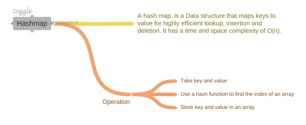
In the realm of data structures, hash maps stand as champions of efficiency when it comes to managing key-value relationships. They offer lightning-fast access retrieval, and storage capabilities, making them indispensable assets for developers across various programming languages.
Here’s a closer look at how hash maps work and their unique advantages:
Unlocking the Abstract: Hash maps provide a concrete implementation of the abstract data type known as an associative array. This means they bring the theoretical concept of key-value associations to life, allowing you to directly harness their power in your code.
Hashing for Efficiency: At the heart of hashmaps lies a clever mechanism called hashing. It transforms keys (like strings or integers) into numerical indices, guiding the storage and retrieval of values within an internal array-like structure. This strategic mapping unlocks incredibly fast access time.
Java’s Hash Map: Your Key to Success: In Java, the
HashMapclass reigns supreme as the go-to implementation for hash maps. It offers a robust and versatile toolkit for managing key-value pairs, boasting exceptional performance for insertion, deletion, and lookup operations.Beyond Arrays: Unleashing Advanced Functionalities: While arrays can handle simple key-value relationships, hash maps offer far greater flexibility and efficiency, especially when dealing with large datasets or complex data structures. They’re optimised for rapid retrieval and modification of values based on their associated keys.
Time and Space Complexity for Hash Map
In the world of data structures, hash maps are renowned for their efficiency, but understanding their time and space complexities is crucial for optimal usage.
Here’s a breakdown of how hash maps manage time and space, ensuring lightning-fast operations in most cases:
Time Complexity: A Tale of Two Scenarios
Average-Case Bliss: Under typical conditions, hash maps operate with a near-magical time complexity of O(1) for insertion, lookup, and deletion. This means they execute these operations in constant time, regardless of the number of key-value pairs stored. It’s like finding a book in a vast library using its exact shelf number - no need for lengthy searches!
Waste-Case Caution: While rare, worst-case scenarios can occur when hash collisions are abundant, leading to potential O(n) time complexity. This means performance might temporarily dip and become proportional to the hash map’s size. However, careful design and collision resolution strategies can effectively mitigate this risk.
Space Complexity: A Linear Relationship
Storing the Goods: Hash maps typically exhibit O(n) space complexity, meaning the space required grows linearly with the number of key-value pairs. Each pair occupies a constant amount of space, ensuring predictable memory usage.
Operations in Action:
Insertion: New key-value pairs are swiftly added by hashing the key to determine its index within the hash map’s internal array-like structure. If a collision arises, a well-crafted collision resolution strategy efficiently handles it.
Deletion: Removing a key-value pair involves hashing the key to pinpoint its index and then gracefully removing the associated item. Again, collision resolution might be needed to maintain a tidy hash map.
Lookup: Retrieving a value based on its key is a breeze. The hash map hashes the key to find its index and swiftly returns the corresponding value.
In conclusion, hash maps offer exceptional performance in most cases, making them invaluable for various applications.
Building a Bulletproof Hash Table: Speed, Smarts, and Avoiding Crash Collisions
Hash tables reign supreme in the world of data structures, offering lighting-fast access to your precious key-value pairs. But building truly exceptional hash tables requires mastering two superpowers: speed and smart collision avoidance.
Speed Demon Hash Codes
Every hash table operation hinges on the blazing-fast computation of hash codes. Think of them as magic fingerprints for your kets, guiding them to their rightful place in the table. A well-designed hash function is the secret sauce to generating these unique identifiers in a flash.
The Collision Conundrum
Imagine two guests arriving at the same hotel room - that’s a collision! In the world of hash tables, it happens when different keys have the same hash code, leading to chaos and confusion. To avoid this data mosh pit, we need effective collision resolution strategies. Think of them as skilled concierges, gracefully assigning alternative rooms to our colliding keys and ensuring everyone has a happy stay.
Taming the Torrent: Collision Resolution in Distributed Hash Tables for Scalable Data Management
In the bustling world of hash maps, collisions are inevitable. They’re like traffic jams on the data highway, slowing down your key-value operations. But fear not! Skilled engineers have devised clever strategies to navigate these roadblocks and keep your hash maps humming along smoothly.
Here’s a peek into the collision resolution toolkit:
Chaining: The Traffic Lights of Hashing:
Imagine each array index as a lane on a busy road. Chaining transforms these lanes into mini-parking lots, using linked lists (or other data structures) to accommodate multiple values with the same hash code. When a collision occurs, it’s like adding a new car to the appropriate parking lot, ensuring everyone has a spot.
Open Addressing: The Art of Finding a Spot:
This approach takes a different route, scanning the entire array for the next available parking space (empty slot) when a collision happens. It’s like a savvy driver circling the block, strategically exploring different options.
Linear Probing: The methodical driver, checking each consecutive space in turn.
Quadratic Probing: The adventurous driver, using a quadratic formula to explore spaces in a more unpredictable pattern.
Double Hashing: The tech-savvy driver, relying on a secondary hash function to determine a unique step size between probes, spreading out the search for a perfect spot.
The Hash Function: Your Traffic Planner:
The heart of collision prevention lies in designing a good hash function. It’s like a skilled urban planner, crafting distinct hash codes (addresses) for different inputs, ensuring traffic flows smoothly across the entire hash map. A well-designed hash function distributes values evenly, minimising the risk of congestion.
Sum It Up: Algorithmic Adventures with Two Numbers
The Two Sum problem stands as a classic computational challenge: given an array of numbers and a target value, your mission is to find all pairs of elements within the array that add up to the target. It's like being a detective tasked with uncovering hidden partnerships among these numbers, where their combined power equals the coveted target.
This seemingly simple yet intriguing problem demands clever algorithmic thinking and understanding of data structures to achieve efficiency. In the upcoming sections, we'll delve into various approaches to conquering the Two Sum challenge, unlocking the secrets of swift and elegant solutions.
Problem Statement
Given an array of integers nums and an integers target, return the indices of the two numbers such that they add up to the target.
Example 1:
Input: nums = [3,2,4,8], target = 12
Output: [2, 3]
Example 2:
Input: nums = [5,5], target = 10
Output: [0,1]
Solution
Hash maps, the champions of lightning-fast key-value associations, offer a powerful solution to the Two Sum problem. Here’s how they elegantly reveal hidden number pairs that sum to the target:
Constructing the Number Playground:
We start by creating an empty hash map, a virtual playground where numbers will mingle and find their matches. This map acts as a swift matchmaker, storing each number’s value and its corresponding index within the array.
Traversing the Array, Seeking Harmony:
We then embark on a journey through the array, examining each number with intent. For every number we encounter:
Calculating the Complement: We determine its complement, the missing piece that would complete the target sum. It’s like seeking the perfect dance partner to achieve a harmonious balance.
Checking for a Match in the Map: We eagerly consult the hash map, asking, “Have you seen this complement before?” If it’s already present, we’ve found a match! The hash map swiftly reveals the index of the complement, and we triumphantly return the indices of the two numbers that fulfil the target sum.
Introducing New Numbers to the Map: If the complement isn’t found, we introduce the current number and its index to the hash map, expanding the pool of potential matches for future encounters.
Java Code: Harnessing the Power of HashMaps:
import java.util.HashMap;

public class TwoSumSolver {
    public static int[] twoSum(int[] nums, int target) {
        HashMap<Integer, Integer> numberMap = new HashMap<>();

        for (int i = 0; i < nums.length; i++) {
            int complement = target - nums[i];

            if (numberMap.containsKey(complement)) {
                // Found the pair!
                return new int[] {numberMap.get(complement), i};
            }

            // Store the current number and its index for future matches
            numberMap.put(nums[i], i);
        }

        // No solution found
        return new int[] {};
    }

    public static void main(String[] args) {
        int[] numbers = {2, 7, 11, 5, 15, 30};
        int targetSum = 12;
        int[] result = twoSum(numbers, targetSum);

        System.out.println("Indices of the two numbers that add up to " + targetSum + ": " + Arrays.toString(result));
    }
}
Time and Space Complexity: The Efficiency Trade-Off
Time Complexity: O(n) This approach enjoys a linear time complexity, meaning its execution time grows directly proportional to the array's size. We only need a single pass through the array, thanks to the hash map's lightning-fast lookups.
Space Complexity: O(n) The space complexity also scales linearly with the array's size due to the storage of elements and their indices within the hash map. This trade-off is often acceptable for the significant speed gains achieved.
Wrapping Up our Hash Map Journey: From Theory to Two Sum Triumph!
In this adventure, we unravelled the secrets of hash maps, exploring their efficient key-value associations and impressive adaptability. We learned how they map keys to specific locations in an array, enabling lightning-fast retrieval and manipulation of data.
Beyond the basics, we delved into crucial considerations for crafting optimal hash functions, ensuring your keys find their rightful homes without getting tangled in collisions. We saw how a well-designed hash function minimises these roadblocks, keeping your hash map running smoothly.
Finally, we put our hash map knowledge to the test by tackling the intriguing Two Sum problem. We witnessed how this data structure becomes a powerful tool for identifying hidden pairs of numbers that sum to a specific target. With hash maps as our weapon, we unlocked an elegant and efficient solution, demonstrating their practical value in solving computational challenges.
This is just the beginning of your hash map exploration! Keep learning, experimenting, and applying these versatile structures to your coding endeavours. Remember, the world of data algorithms awaits, and hash maps are your trusty companions on this thrilling journey.
Happy coding and unlocking new algorithmic mysteries!